Fit Extinction Curves

The dust_extinction package is built on the astropy.modeling package. Fitting is done in the standard way for this package where the model is initialized with a starting point (either the default or user input), the fitter is choosen, and the fit performed.

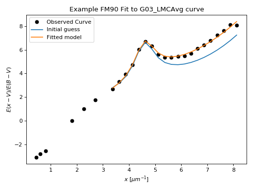
Example: FM90 Fit

In this example, the FM90 model is used to fit the observed average extinction curve for the LMC outside of the LMC2 supershell region (G03_LMCAvg dust_extinction model).

import matplotlib.pyplot as plt
import numpy as np

from astropy.modeling.fitting import LevMarLSQFitter

from dust_extinction.dust_extinction import G03_LMCAvg, FM90

# get an observed extinction curve to fit
g03_model = G03_LMCAvg()

x = g03_model.obsdata_x
# convert to E(x-V)/E(B0V)
y = (g03_model.obsdata_axav - 1.0)*g03_model.Rv
# only fit the UV portion (FM90 only valid in UV)
gindxs, = np.where(x > 3.125)

# initialize the model
fm90_init = FM90()

# pick the fitter
fit = LevMarLSQFitter()

# fit the data to the FM90 model using the fitter
#   use the initialized model as the starting point
g03_fit = fit(fm90_init, x[gindxs], y[gindxs])

# plot the observed data, initial guess, and final fit
fig, ax = plt.subplots()

ax.plot(x, y, 'ko', label='Observed Curve')
ax.plot(x[gindxs], fm90_init(x[gindxs]), label='Initial guess')
ax.plot(x[gindxs], g03_fit(x[gindxs]), label='Fitted model')

ax.set_xlabel('$x$ [$\mu m^{-1}$]')
ax.set_ylabel('$E(x-V)/E(B-V)$')

ax.set_title('Example FM90 Fit to G03_LMCAvg curve')

ax.legend(loc='best')
plt.tight_layout()
plt.show()

(Source code, png, hires.png, pdf)

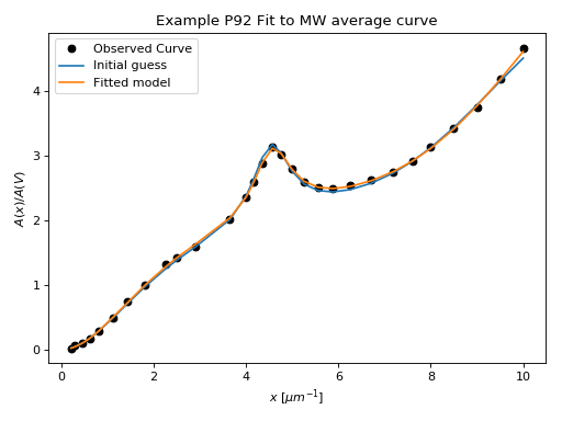
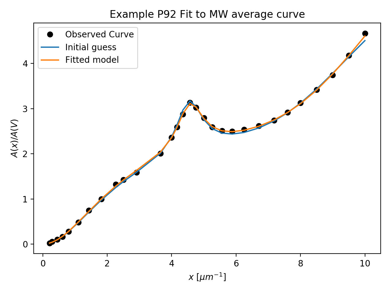
Example: P92 Fit

In this example, the P92 model is used to fit the observed average extinction curve for the MW as tabulted by Pei (1992).

import matplotlib.pyplot as plt
import numpy as np

from astropy.modeling.fitting import LevMarLSQFitter

from dust_extinction.dust_extinction import P92

# Milky Way observed extinction as tabulated by Pei (1992)
MW_x = [0.21, 0.29, 0.45, 0.61, 0.80, 1.11, 1.43, 1.82,
        2.27, 2.50, 2.91, 3.65, 4.00, 4.17, 4.35, 4.57, 4.76,
        5.00, 5.26, 5.56, 5.88, 6.25, 6.71, 7.18, 7.60,
        8.00, 8.50, 9.00, 9.50, 10.00]
MW_x = np.array(MW_x)
MW_exvebv = [-3.02, -2.91, -2.76, -2.58, -2.23, -1.60, -0.78, 0.00,
             1.00, 1.30, 1.80, 3.10, 4.19, 4.90, 5.77, 6.57, 6.23,
             5.52, 4.90, 4.65, 4.60, 4.73, 4.99, 5.36, 5.91,
             6.55, 7.45, 8.45, 9.80, 11.30]
MW_exvebv = np.array(MW_exvebv)
Rv = 3.08
MW_axav = MW_exvebv/Rv + 1.0

# get an observed extinction curve to fit
x = MW_x
y = MW_axav

# initialize the model
p92_init = P92()

# pick the fitter
fit = LevMarLSQFitter()

# fit the data to the P92 model using the fitter
#   use the initialized model as the starting point
#   accuracy set to avoid warning the fit may have failed
p92_fit = fit(p92_init, x, y, acc=1e-3)

# plot the observed data, initial guess, and final fit
fig, ax = plt.subplots()

ax.plot(x, y, 'ko', label='Observed Curve')
ax.plot(x, p92_init(x), label='Initial guess')
ax.plot(x, p92_fit(x), label='Fitted model')

ax.set_xlabel('$x$ [$\mu m^{-1}$]')
ax.set_ylabel('$A(x)/A(V)$')

ax.set_title('Example P92 Fit to MW average curve')

ax.legend(loc='best')
plt.tight_layout()
plt.show()

(Source code, png, hires.png, pdf)